Edge Machine Learning: Architectures, Quantization, and On-Device Inference
A technical deep dive into deployment paradigms for machine learning on edge hardware, exploring quantization techniques, hardware accelerators, memory constraint management, and runtime execution frameworks.

Machine learning (ML) has traditionally relied on high-performance cloud infrastructure equipped with clusters of high-power GPUs. However, reliance on centralized server topologies introduces critical failure points for systems requiring real-time responsiveness, deterministic latency, strict data privacy, or operation in bandwidth-constrained environments.
Edge Machine Learning (Edge ML)—often referred to as TinyML when deployed on ultra-low-power microcontrollers—shifts the inference workload from the cloud directly to end-node devices. These hardware platforms range from application-class System-on-Chips (SoCs) and Edge Neural Processing Units (NPUs) down to 32-bit microcontrollers operating within milliwatt power budgets.
Deploying neural networks to target environments with constrained RAM (ranging from kilobytes to megabytes) and tight thermal envelopes requires a fundamental shift in model architecture design, mathematical representation, and execution runtime strategies.
The Hardware Spectrum of Edge Inference
Edge inference hardware exists on a continuous spectrum defined by compute capacity, memory architecture, power consumption, and hardware acceleration capabilities.
+-------------------------------------------------------------------------+
|                              EDGE HARDWARE                              |
+------------------------------------+------------------------------------+
|         Microcontrollers           |        Application SoCs            |
|     (Cortex-M, RISC-V, ESP32)      |     (Cortex-A, Edge NPUs/TPUs)    |
|  SRAM: 64 KB - 2 MB                |  RAM: 1 GB - 16 GB                 |
|  Power: 1 mW - 500 mW              |  Power: 2 W - 25 W                 |
|  Ops: Fixed-point SIMD             |  Ops: Dedicated Tensor Cores       |
+------------------------------------+------------------------------------+
1. Microcontrollers (MCUs)
Operating within sub-watt power envelopes, 32-bit microcontrollers (such as ARM Cortex-M, ESP32, or RISC-V cores) feature severely limited static RAM (typically 64 KB to 2 MB) and execute code directly from flash memory. Inference on MCUs relies heavily on SIMD (Single Instruction, Multiple Data) extensions, such as ARM CMSIS-NN instructions, which accelerate 8-bit integer operations using vector packed math.
2. Application Processors and Edge SoCs
Higher-tier edge systems (such as single-board computers and industrial gateways) combine multi-core application processors (ARM Cortex-A series, RISC-V 64-bit) with dedicated hardware accelerators like Neural Processing Units (NPUs) or integrated Vector Processing Units (VPUs). These engines utilize specialized matrix multiplication arrays capable of sustaining trillions of operations per second (TOPS) per watt.
Hardware Architecture Comparison
| Platform Class | Typical Memory | Target Power | Primary Compute Acceleration | Deployment Target |
|---|---|---|---|---|
| Ultra-Low Power MCU | 64 KB – 512 KB SRAM | 1 mW – 100 mW | Single-core SIMD / DSP Instructions | Keyword spotting, sensor anomaly detection |
| Advanced MCU / Dual Core | 1 MB – 8 MB SRAM/PSRAM | 100 mW – 1 W | Vector Extensions, Low-clock MAC units | Audio processing, low-res visual wake words |
| Edge Application SoC | 1 GB – 16 GB LPDDR | 2 W – 15 W | Multi-core NPU / Integrated GPU | Multi-stream object detection, pose estimation |
| Industrial Edge AI Node | 8 GB – 32 GB LPDDR/DRAM | 15 W – 60 W | Discrete Tensor Cores / PCIe NPUs | Real-time industrial automation, high-FPS vision |
Model Compression and Optimization Paradigms
Deep learning architectures trained in native floating-point precision ($FP32$ or $FP16$) are structurally unviable for bare-metal edge execution due to memory footprint size and the high clock-cycle cost of floating-point arithmetic units (FPUs). Transitioning models from training environments to edge hardware requires targeted optimization techniques.
Quantization Mechanics
Quantization reduces the bit-width of model weights and activation tensors, typically converting 32-bit floating-point ($FP32$) numbers into 8-bit integers ($INT8$) or sub-byte formats ($INT4$).
The fundamental uniform affine quantization mapping function translates a continuous real value $r$ to a discrete integer value $q$:
$$q = \text{round}\left(\frac{r}{S}\right) + Z$$
Where:
- $S$ (Scale) is a positive real float determining the resolution of the quantization bin.
- $Z$ (Zero-Point) is an integer value mapping the real value $0.0$ to its quantized equivalent, ensuring that zero-padding operations do not introduce precision distortion.
De-quantization reverses this transformation during execution steps when higher precision accumulation is required:
$$r = S \cdot (q - Z)$$
Post-Training Quantization (PTQ) vs. Quantization-Aware Training (QAT)
- Post-Training Quantization (PTQ): Operates directly on a fully trained $FP32$ model using a small calibration dataset to evaluate the dynamic dynamic range of activation tensors across key layers. PTQ is computationally lightweight but can cause accuracy degradation in networks with sensitive activation distribution profiles (e.g., MobileNet depthwise separable convolutions).
- Quantization-Aware Training (QAT): Simulates quantization noise during the forward pass of model training using fake-quantization nodes. Gradients are computed in $FP32$ using straight-through estimators (STE) during backpropagation. QAT allows the network weights to adjust to lower precision bounds, minimizing accuracy degradation even when targeted at $INT8$ or $INT4$ representations.
       POST-TRAINING QUANTIZATION (PTQ)
Train (FP32) ---> Calibrate Datasets ---> Quantize Weights & Activations (INT8)

       QUANTIZATION-AWARE TRAINING (QAT)
Train with Fake-Quantization Nodes (FP32/INT8 mix) ---> Convert directly to INT8 Target Engine
Pruning: Structural vs. Unstructured
Pruning eliminates redundant parameters within the weight matrices:
- Unstructured Pruning: Sets individual weight scalars below a chosen threshold to zero. While achieving high theoretical sparsity, unstructured pruning rarely improves execution latency on general-purpose hardware unless the underlying compiler and hardware engine explicitly support sparse matrix operations.
- Structured Pruning: Removes entire channels, kernels, or residual blocks. This alters the dimensional structure of tensors, yielding direct latency reductions and memory footprint savings on standard matrix processing units without requiring specialized sparse hardware kernels.
Knowledge Distillation
Knowledge distillation uses a large, over-parameterized "teacher" model to guide the training of a compact, memory-efficient "student" model. The student is trained on a loss function composed of cross-entropy against hard ground-truth labels and Kullback-Leibler (KL) divergence against the soft output probability distributions generated by the teacher model:
$$\mathcal{L}{total} = (1 - \alpha) \mathcal{L}{CE}(y, \hat{y}{student}) + \alpha \tau^2 \mathcal{L}{KL}\left( \text{softmax}\left(\frac{z_{teacher}}{\tau}\right), \text{softmax}\left(\frac{z_{student}}{\tau}\right) \right)$$
Where $\tau$ represents the soft-label temperature parameter and $\alpha$ balances the loss weight.
Edge Runtime Execution Frameworks
Standard deep learning frameworks (such as PyTorch or TensorFlow) rely on dynamic memory allocation, expansive standard C++ libraries, and non-deterministic kernel execution engines unsuitable for resource-constrained edge systems. Edge inference relies on specialized runtimes.
Key Runtimes
- TensorFlow Lite for Microcontrollers (TFLM): Designed specifically for bare-metal microcontrollers. It eliminates dependencies on dynamic memory allocation (
malloc), relying instead on a pre-allocated byte array known as a tensor arena. - ONNX Runtime Mobile / Micro: Executes Open Neural Network Exchange graph representations optimized for mobile devices and embedded platforms.
- ExecuTorch: PyTorch's native light-weight runtime targeting deployment across mobile and edge hardware, enabling step-down compilation directly from PyTorch eager-mode graphs.
- MicroTVM: An open-source tensor compiler framework that translates high-level model definitions into bare-metal, target-specific C code kernels optimized for specific microcontroller instruction sets.
Memory Arena Allocation Patterns
To guarantee execution stability on resource-constrained microcontrollers, runtimes utilize static static memory scheduling. The memory arena must accommodate model parameters, intermediate tensor activations, and runtime state without dynamic dynamic heap allocation.
+--------------------------------------------------------------------+
|                        TENSOR ARENA (RAM)                          |
+-------------------+------------------------------------------------+
| Runtime Handles   | Activation Buffer Overlays (Scratchpad Memory) |
| & Tensor Headers  | Tensor A -> Tensor B -> Output                 |
+-------------------+------------------------------------------------+
The scratchpad memory uses lifetime analysis of nodes in the computational graph: memory assigned to Tensor A is safely overwritten by Tensor C once Tensor A is no longer required by downstream operators.
Technical Example: Preparing and Running an Edge Model Pipeline
Below is an execution model workflow demonstrating how a PyTorch model is converted, quantized, and initialized in a C++ edge runtime environment using TFLM-style static memory patterns.
Step 1: Exporting and Quantizing (Python Workflow)
import torch
import torch.nn as nn

# Define a lightweight feedforward topology
class EdgeModel(nn.Module):
    def __init__(self):
        super(EdgeModel, self).__init__()
        self.fc1 = nn.Linear(16, 32)
        self.relu = nn.ReLU()
        self.fc2 = nn.Linear(32, 4)

    def forward(self, x):
        return self.fc2(self.relu(self.fc1(x)))

model = EdgeModel()
model.eval()

# Example trace export for ONNX / Edge runtime consumption
dummy_input = torch.randn(1, 16)
torch.onnx.export(
    model,
    dummy_input,
    "edge_model.onnx",
    input_names=['input'],
    output_names=['output'],
    dynamic_axes=None  # Static tensor dimensions required for embedded targets
)
Step 2: C++ Embedded Execution Patterns (Static Arena Allocation)
The following C++ snippet demonstrates static memory provisioning for bare-metal execution environments.
#include "tensorflow/lite/micro/micro_interpreter.h"
#include "tensorflow/lite/micro/micro_mutable_op_resolver.h"
#include "tensorflow/lite/schema/schema_generated.h"

// Define fixed memory allocation for the tensor arena (e.g., 64KB)
constexpr int kTensorArenaSize = 64 * 1024;
alignas(16) uint8_t tensor_arena[kTensorArenaSize];

// External reference to model byte array compiled into flash memory
extern const unsigned char g_edge_model_data[];

void InitAndRunInference(const float* input_data, float* output_data) {
    // Map the model flatbuffer schema from Flash memory
    const tflite::Model* model = tflite::GetModel(g_edge_model_data);

    // Instantiate specific operators to minimize binary size footprint
    tflite::MicroMutableOpResolver<2> resolver;
    resolver.AddFullyConnected();
    resolver.AddRelu();

    // Construct the micro interpreter with zero dynamic heap calls
    tflite::MicroInterpreter interpreter(
        model, resolver, tensor_arena, kTensorArenaSize);

    // Allocate memory blocks inside the tensor arena for model ops
    TfLiteStatus allocate_status = interpreter.AllocateTensors();
    if (allocate_status != kTfLiteOk) {
        return; // Allocation failure (Arena size insufficient)
    }

    // Assign input buffer pointers
    TfLiteTensor* input = interpreter.input(0);
    for (size_t i = 0; i < 16; ++i) {
        input->data.f[i] = input_data[i];
    }

    // Run linear graph execution
    TfLiteStatus invoke_status = interpreter.Invoke();
    if (invoke_status != kTfLiteOk) {
        return; // Kernel execution failure
    }

    // Extract output pointers
    TfLiteTensor* output = interpreter.output(0);
    for (size_t i = 0; i < 4; ++i) {
        output_data[i] = output->data.f[i];
    }
}
Common Pitfalls and Engineering Bottlenecks
1. Dynamic Shape Operations
Edge compilers require fully static computational graphs. Operators reliant on dynamic shape inputs at runtime—such as dynamic string parsing, spatial transformer networks with unbounded batch sizes, or dynamic sequence lengths in RNNs/Transformers—will fail kernel compilation steps or force costly execution fallbacks to slow software emulation engines.
2. Operator Fallback Overheads
If a specific neural network layer (e.g., specialized activation functions like GELU or custom Einstein-sum operations) lacks native optimization within an NPU's vendor SDK or SIMD kernel library, execution falls back to generic CPU emulation. This introduces kernel invocation overhead, memory swapping, and significant latency spikes.
3. Memory Bus Saturations vs. Compute Bottlenecks
On edge devices, compute engines (ALUs/MAC units) often outpace the memory bus bandwidth available to fetch model weights from external SPI Flash or PSRAM. This condition, known as being memory-bound, means latency optimizations must focus on reducing data transfer sizes (e.g., aggressive weight quantization) rather than simply reducing floating-point operational counts (FLOPs).
4. Thermal Throttling
Continuous edge ML execution on fanless, enclosed hardware (such as smart cameras or wearable health monitors) can induce rapid thermal buildup. Modern application processors mitigate thermal runaway by dynamically lowering core clock frequencies (thermal throttling), causing sudden non-deterministic variance in inference latency.
Frequently Asked Questions
How does integer quantization preserve accuracy in complex models?
Integer quantization preserves operational accuracy by mapping dynamic execution values across non-linear layer outputs into discrete scaled range channels. Techniques such as per-channel quantization (assigning unique scale $S$ and zero-point $Z$ parameters to each individual convolutional filter channel rather than the entire tensor layer) prevent out-of-range precision loss caused by outlier activation peaks.
Can custom operators be integrated into light runtime engines like TFLM?
Yes. Custom operators can be introduced by writing specialized operator kernel files in C++. This requires implementing standard interface functions: Init() for state allocation, Prepare() to calculate and validate output tensor shapes, and Eval() to execute the target algorithm using optimized assembly instructions (such as inline SIMD).
What is the primary difference between zero-point and scale in INT8 representations?
Scale ($S$) is a positive real dynamic number representing the step-size difference between adjacent integer values in floating-point space. Zero-point ($Z$) is an exact int8 offset value matching real-world floating-point value $0.0$. The presence of zero-point allows asymmetric quantization, which efficiently handles skewed activation functions like ReLU where all values are non-negative.
Why is static dynamic memory allocation strictly enforced on tiny edge runtimes?
Static memory allocation prevents non-deterministic memory fragmentation and dynamic heap allocation failures (out-of-memory faults) during prolonged continuous runtime cycles. By pre-allocating a continuous block of memory (the tensor arena) at startup, execution guarantees deterministic operational predictability and zero dynamic overhead on embedded microcontrollers.
Summary and Next Steps
Deploying machine learning models to edge targets requires managing constraints across compute capacity, memory access, power consumption, and deterministic performance. Successful edge ML implementations depend on:
- Matching network topologies to the specific hardware hardware capabilities of the target platform (MCU SIMD vs. dedicated NPU).
- Applying aggressive optimization techniques, such as static INT8/INT4 quantization, channel-structured pruning, and knowledge distillation.
- Structuring software architectures around bare-metal runtimes using static tensor memory patterns to avoid dynamic heap allocation.
To begin building edge ML applications, experiment with compiling simple neural networks using TensorFlow Lite for Microcontrollers or MicroTVM, targeting low-cost embedded platforms such as ARM Cortex-M or ESP32 development boards.